Google Sheets MCQs
Google Sheets MCQs
Answer these 40 Google Sheets MCQs and assess your grip on the subject of Google Sheets.
Scroll below and get started!
Choose True or False.
If you have Google Drive installed on your computer and you are creating a spreadsheet in the Google Drive on the web, then the spreadsheet will also be automatically saved to your local hard drive.
A.
True
B.
False

A.
(i)
B.
(ii)
C.
(iii)
D.
(iv)
3: Which of the following statements about Annotations in Google Sheets is correct?
A. Annotations are the text notes that can be attached to charts.
B. Annotations are the text notes that can be attached to images.
C. Annotations are the text notes that can be attached to comments.
D. Annotations are the text notes that can be attached to drawings.
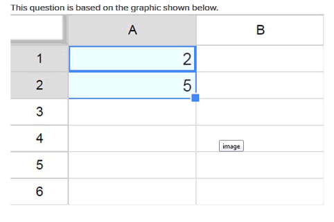
The sum of squares of numbers 10, 12. and values of cells from B2 to B4 is to be generated in a GoogleSheets spreadsheet. Which of the following is/are the correct form of the function to be used to generate the sum?
1. =SUMSQ(10,12,82-84)
2. =SUMSQ (10.12.82.84)
3. =SUMSO(B2:B4,10,12)
4. =SUMSQ(10,12.82:B4)
A.
Only option 4 is correct.
B.
Both options 1 and 4 are correct.
C.
Both options 3 and 4 are correct.
D.
Both options 2 and 4 are correct.
5: Which of the following is correct regarding movement of a row in Google Sheets?
A. If a row is dragged and moved to a new location in a spreadsheet, the row at the target location and the rows above it get shifted one position up.
B. A single row can be moved but a group of subsequent rows cannot be moved in a spreadsheet.
C. If a row is moved to the location of another row in a spreadsheet. both rows get swapped.
D. A row can be moved at the most ten positions below its current position in a spreadsheet.
6: Which of the following actions can be performed with Google Sheets using Google Drive?
A. You can import and convert .xls. .xlsx, .csv, .txt and .ods formatted data to a Google spreadsheet.
B. You can export .xls, .xlsx, .csv, .txt and .ods formatted data, as well as PDF and HTML files.
C. You can use formula editing to perform the calculations.
D. You can embed the spreadsheet on a blog or a website.
E. All of the above.
7: Which of the following options should be used if you want to name a range of cells in a Google Sheets spreadsheet?
A. Click on Data menu on the menu bar -> Select Named Ranges option -> Enter a desired name and click Done button.
B. Click on Insert menu on the menu bar -> Select Named Ranges option -> Enter a desired name and click Done button.
C. Click on View menu on the menu bar -> Select Named Ranges option -> Enter a desired name and click Done button.
D. Such a feature is not available in Google Sheets.
8: Jenny wants to store a phone number in the format of plus sign followed by the number in a GoogleSheets spreadsheet(i.e., +012734343344). But when she directly enters phone number as+012734343344 in a cell in the spreadsheet. it gets converted to 012734343344. What can she do to enter the telephone number in the desired format?
A. Begin the telephone number with a single quote. Example: '+012734343344
B. Use function CONCATENATE Example: =CONCATENATE("+",012734343344)
C. Click Format menu on the menu bar > Select Number option > Select More Formats option > Click Custom number format... option and select the format +#, ##O_) ;( $#, ##0)
D. Any of the above options can be used.
9: In order to insert an image inside a particular cell in a Google Sheets spreadsheet. which of the following options can be used?
A. The image is inserted using IMAGE function.
B. Click on the cell in which you wish to insert the image -> Click on the Insert menu option on the menu bar —> Click Image... option -> Click button Choose an image to upload —> Select the image and click Open.
C. Right click on the cell in which you wish to insert the image -> Select image... option from context menu -> Click button Choose an image to upload -> Select the image and click Open.
D. Any of the above options can be used.
A.
6. 7. 8, and 9
B.
2. 2. 2. and 2
C.
5. 5. 5. and 5
D.
8.11.14. and 17
E.
4. 5. 6. and 7
A.
Only options 2, 3 and 4
B.
Only options 1, 2 and 3
C.
Only option 3
D.
Only option 2
12: By default. what kind of cell reference is used in Google Sheets?
A. Relative reference
B. Absolute reference
C. Mixed reference
13: In which of the following views of Google Sheets spreadsheet are we not able to select cells. Rename sheets or charts using Google Drive on the web?
A. Normal spreadsheet
B. List
C. Gridline
D. All of the above.
14: Peter entered a value 1041 in a cell and it automatically got converted to the date format by Google Sheets. Which of the following options should he select to avoid this automatic conversion?
A. Click on the Format menu on the menu bar > Select Number option > Click Plain Text option.
B. Click on the Format menu on the menu bar > Select Number option > Click Automatic option.
C. Click on the Format menu on the menu bar > Select Number option > Click Number option.
D. Click on the Data menu on the menu bar > Select Number option > Click Number option.

A.
To apply border to a table.
B.
To change direction of text from right to left in a cell.
C.
To change direction of spreadsheet grid from right to left.
D.
To create new Filter view.
16: In Google Sheets. which of the following keyboard shortcuts is used to add a line break within a cell for a Windows system?
A. Ctrl + Enter
B. Alt + Enter
C. Ctrl + L
D. Both options a and b can be used
17: John selects and copies a column D10:D13 in Google Sheets. While pasting the contents to cell H8. he selects option Paste special > Paste transpose. Which of the following is correct about pasted contents?
A. The contents of D10:D13 will be copied to H8:H11.
B. The contents of D10:D13 will be reversed and copied to H8:K8.
C. The contents of D10:D13 will be copied to H8:K8.
D. The contents of D10:D13 will be added up and their average will be pasted in cell H8.
18: If you want to store values 13. 25,100. and 23 in cells A1. A2. A3. and A4 respectively; then which of the following array formats should you be entering in cell A1 to obtain the desired result?
A. = [13; 25; 100; 23]
B. =[13. 25,100.23}
C. = (13: 25: 100: 23)
D. = (13.25.100.23)
19: If a cell is copied and pasted to new cell using Paste special > Paste format only option in Google Sheets, what will happen to the new cell?
A. Only the cell formatting will be pasted in the new cell and not the values or formulas from the copied cell.
B. Only conditional formatting will be pasted in the new cell from the copied cell.
C. Borders, if any, applied on the copied cell will not be applied to the new cell.
20: Which of the following would you use if you want different people to view the data differently in your spreadsheet in Google Sheets?
A. Filter
B. Pivot table
C. Filter views..
D. View
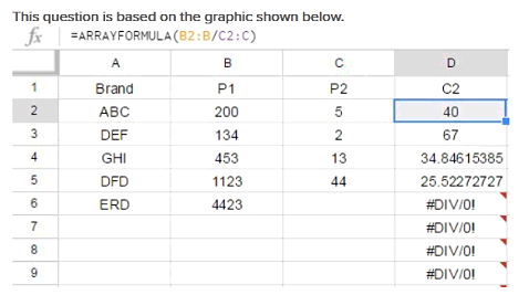
A.
NA(ARRAYFORMULA(B2:B/C2:C))
B.
ISERROR(ARRAYFORMULA(82:B/C2:C))
C.
ARRAYFORMULAlIFERROR((82:B/C2:C))
D.
There is no solution to this problem as ARRAYFORMULA does not accept an empty second
parameter.

A.
Select the pie chart and click on the small arrow button on the upper right corner of the chart >
Click Advanced Edit... option > Click Chart types tab > Click Doughnut chart option under the Pie Label.
B.
Select the pie chart and click on the formula bar and write function = VALUE (B2, B3, B4) where 82. 83 and B4 are the fields containing sales of cars ABC. NEW and BEE respectively.
C.
Select the pie chart and click on the small arrow button on the upper right corner of the chart >
Click Advanced Edit... option > Click Chart types tab > Select Values option from the drop-down box.
D.
Select the pie chart and click on the small arrow button on the upper right corner of the chart >
Click Advanced Edit... option > Click Customization tab > Select Value option in the drop-down box in front of the Slice label.
23: Which of the following sections of the Report Editor window of Pivot table... menu option is edited for adding a Calculated Field to a pivot table in Google Sheets?
A. Values
B. Columns
C. Rows
D. Filter
24: Which of the following options can be used to resize the height of a row in Google Sheets?
A. Click on Edit menu on the menu bar > Select Resize row... option.
B. Click on Format menu on the menu bar > Select Resize row... option.
C. Click on the header for the row to be resized > Drag cursor to expand selection > Right click and choose Resize row... option.
D. Rows cannot be resized in Google Sheets.
25: What is the correct function to be used if you want to replicate and copy data from A2 cell of a sheet called Sheet number 4 to some other sheet within the same spreadsheet in Google Sheets?
A. =‘Sheet number 4'A2'
B. =‘Sheet number 4'IA2
C. =Sheet number 4’A2
D. =Sheet number 4!'A2'
26: In Google Sheets. which of the following functions works only on a sorted row or column?
A. VLOOKUP
B. LOOKUP
C. MATCH
D. HLOOKUP
Choose True or False.
A spreadsheet uploaded on Google Drive can be edited only when it has been converted to Google Sheets format.
A.
True
B.
False
Which of the following operations are possible in the forms created using Google Drive?
1. Edit
2. Delete
3. Duplicate
A.
1 and 2 only
B.
2 and 3 only
C.
1 and 3 only
D.
1, 2 and 3
29: Which of the following functions is used to return the current date and time in Google Sheets?
A. TODAY()
B. WORKDAY()
C. Now()
D. Both options a and c can be used
Choose the incorrect statement from the following statements.
You can change the number, date or currency formats in your spreadsheet created using Google Drive.
A.
You can add formulas in your spreadsheet created using Google Drive.
B.
You cannot wrap text in your spreadsheet created using Google Drive.
C.
You can insert comments in your spreadsheet created using Google Drive.
31: In Google Sheets. which of the following options would you select if you want to keep the first row of a spreadsheet visible even when you scroll down to the 250th row of the same spreadsheet?
A. Lock
B. Freeze
C. Static
D. Tracker

A.
(i)
B.
(ii)
C.
(iii)
D.
(iv)
33: In google Sheets, conditional cell formatting can be done on the basis of which of the following?
A. Value
B. Formula
C. Image
D. Both options a and b
34: In Google Sheets, which of the following options is not available to a user who has editing permission on a protected sheet?
A. Set editing permission for protected sheet/range.
B. Make a copy of the spreadsheet.
C. Removing editing permission for owners.
D. None of the above.
35: Which of the following options will you choose to protect a sheet or a range in Google Sheets?
A. Click Data menu on the menu bar > Click Protected Sheets and ranges option.
B. Click View menu on the menu bar > Click Protected Sheets and ranges option.
C. Click Edit menu on the menu bar > Click Protected Sheets and ranges option
D. Click File menu on the menu bar > Click Protected Sheets and ranges option.
36: Peter entered the first and the last names of the employees of his company in single cells separated by a space. In order to separate the first and the last names in two columns, which of the following options should he use?
A. Select the column whose text you wish to split -> Click on Format menu on the menu bar —> Select Text wrapping option -> Select Split text into columns option and select the separator as Space.
B. Select the column whose text you wish to split -> Click on Format menu on the menu bar -> Select Conditional formatting option -> Select Split text into columns option and select the separator as Space.
C. Select the column whose text you wish to split -> Click Data menu on the menu bar —> Select Split text into columns option and select the separator as Space.
D. Select the column whose text you wish to split -> Right Click to open context menu ->Se|ect Split text into columns option and select the separator as Space.
A.
=QUERY(Sheet1!1:1000,"select colA,colB,colD group by COD")
B.
=QUERY(Sheet1!1:1000,"se|ect colD,max(colC) group by colD,colC")
C.
=QUERY(Sheet1!1:1000,"select colD,max(colC) group by colD")
D.
=QUERYlSheet1!1:1000,"select colD,colC group by colD,coIA,colB")
38: Suppose you want to ensure that the values entered in the particular column of a table are between 10 to 50 and any other value. if entered. is rejected or a warning message is displayed by Google Sheets. Which of the following procedures should you use?
A. Click on Format menu on the menu bar -> Select Custom number format option -> Select Criteria as Number and enter values 10 and 50 -> Apply other required settings and click Save.
B. Select the column —> Click on Data menu on the menu bar -> Select Validation... option -> Select Criteria as Number and enter values 10 and 50 -> Apply other required settings and click Save.
C. Click on Format menu on the menu bar -> Select Conditional formatting option -> Select Criteria as Number and enter values 10 and 50 -> Apply other required settings and click Save.
D. Both options b and c can be used.
A. Comment
B. Note
C. Either Comment or Note
D. None of these
40: Which of the following options is correct regarding Find and replace feature in Google Sheets?
A. You cannot search across multiple spreadsheets.
B. You can search within formulas.
C. You can search within specific range.
D. None of the above
41: While performing conditional formatting in a Google Sheets spreadsheet, a test rule containing p’r can format the cells containing which of the following options?
A. pqr
B. pr
C. pqqr
D. Pq
E. Qr
42: Which of the following options allow you to turn off the filter in a Google Sheets spreadsheet?
A. Click Filter icon on the toolbar.
B. Click Data menu on the menu bar > Click Filter option to turn off the filter.
C. Click Tools menu on the menu bar > Click Filter option to turn off the filter.
D. Press keyboard shortcut Ctrl + F.
43: In Google Sheets, which of the following options will allow you to remove all the data validations applied on a worksheet in one go?
A. Select the complete sheet -> Right click anywhere in the sheet —> Select Protect Range... option -> Click Remove validation button.
B. Select the complete sheet —> Click on Data menu on the menu bar —> Select Validation... option —> Click Remove validation button.
C. Select the complete sheet -> Click on Edit menu on the menu bar -> Select Data Validation... option -> Click Reset Iink
D. Select the complete sheet -> Right click anywhere in the sheet -> Select Data Validation... option -> Click Remove validation button.
Suppose you send out a form to others for collecting their responses. If you choose New Google
Forms option for collecting the responses, then which of the following options can be used as the storage destination?
A.
New spreadsheet
B.
Enter in an existing spreadsheet
C.
New sheet in an existing spreadsheet
D.
Keep responses only in Forms
45: Who is allowed to set editing permissions for protected sheets/ranges in Google Sheets?
A. Owner of the spreadsheet
B. Editor
C. Viewer
D. All of the above.
46: A single spreadsheet document is often called a ____.
A. Insert
B. Shareware
C. Worksheet
D. Microsoft Paint
47: Spreadsheets are particularly useful for ____
A. Desktop Publishing
B. Hard disk backup software
C. What If analysis
D. All of the above
List of Google Sheets MCQs Mul...
Available in:
![]() Google Sheets MCQs
Google Sheets MCQs